FTIR spectra normalised to spectral feature
Processing and displaying Fourier-transform infrared (FTIR) spectra, though generally pretty straight-forward, provides some rather hidden obstacles from the perspective of a general data analysis framework. This is due to two aspects of FTIR spectra not common to other spectroscopy data: Spectra are often displayed as transmission, i.e. with “negative” features, and the conventional x axis (in wavenumbers) is inverted.
In this particular example, FTIR spectra for two different samples have been recorded, and we are interested in comparing the spectra normalised to a particular spectral feature in the range of 1680 to 1750 wavenumbers.
To this end, a series of tasks needs to be performed on each dataset:
Import the data (assuming ASCII export)
Correct for DC offset, i.e. perform a baseline correction of 0-th order.
Normalise to the spectral feature used as a reference, but explicitly not to the entire recorded range.
Plot both spectra in one axis for graphical display of recorded data, following the convention in FTIR to plot an inverse x axis.
There are two ways to invert an axis: The preferred method is to explicitly set the axis property (note that you can specify which axis to invert or even both, if you provide a list). Alternatively, shown here as a comment, you can provide axis limits in descending order. While the latter method does do the trick, you need to explicitly provide axis limits in this case. This might, however, not be convenient.
In case of the data used here, the x axis is recorded in descending order. Therefore, for the baseline correction step, the five percent fitting range are taken from the left part in the figure, i.e. at high wavenumbers. Depending on how your data were recorded and how you set your plot initially, this may be confusing and lead to unexpected results.
Note
As mentioned previously, using plain ASpecD usually does not help you with a rich data model of your dataset, containing all the relevant metadata. However, in the case shown here, it nicely shows the power of ASpecD on itself. Currently, there is no ASpecD-based Python package available for FTIR spectra, at least none the author of the ASpecD framework is aware of.
 1format:
 2  type: ASpecD recipe
 3  version: '0.2'
 4
 5datasets:
 6  - source: FTIR-C1_1.csv
 7    label: Substance 1
 8    importer: TxtImporter
 9    importer_parameters:
10      skiprows: 2
11      delimiter: ';'
12  - source: FTIR-C2_1.csv
13    label: Substance 2
14    importer: TxtImporter
15    importer_parameters:
16      skiprows: 2
17      delimiter: ';'
18
19tasks:
20  - kind: processing
21    type: BaselineCorrection
22    properties:
23      parameters:
24        fit_area: [5, 0]
25
26  - kind: processing
27    type: Normalisation
28    properties:
29      parameters:
30        range: [1750, 1680]
31        range_unit: axis
32        kind: minimum
33
34  - kind: multiplot
35    type: MultiPlotter1D
36    properties:
37      properties:
38        axes:
39          # xlim: [4000, 635]
40          invert: x
41          xlabel: '$wavenumber$ / cm$^{-1}$'
42          ylabel: '$normalised\ transmission$'
43      parameters:
44        tight_layout: True
45        show_legend: True
46      filename: ftir-normalised.pdf
47
Result
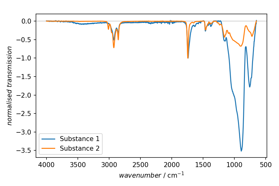
Result of the plotting step in the recipe shown above. The two spectra presented have been normalised to the transmission band between 1680 and 1750 wavenumbers.