You're reading the documentation for a development version. For the latest released version, please have a look at v0.12.
Models: An introduction
Classes used:
Models:
Plotting:
Processing:
Although the primary motivation for the aspecd.model module is to provide mathematical models that can be used for fitting experimental data, in conjunction with the FitPy package, they can be used to create artificial datasets and demonstrate the capabilities of the ASpecD framework.
As there are a few subtle differences between working with actual (imported) data and models, this page serves as an introduction to working with model data.
Working with imported data vs. models
The typical use case of the ASpecD framework, and even more so the packages based on it, is to work with actual data that are imported at the top of the recipe. Hence, a usual recipe will always contain a dataset block near the top with references to the data to import:
 1format:
 2  type: ASpecD recipe
 3  version: '0.3'
 4
 5datasets:
 6  - /path/to/first/dataset
 7  - /path/to/second/dataset
 8
 9tasks:
10  - kind: singleplot
11    type: SinglePlotter1D
Furthermore, whatever task you perform, if you do not explicitly specify via an apply_to directive what datasets the task should be applied to, all of the datasets will be used.
When working with artificial data generated via models, two things are different:
You do not need a
datasetblock, although you can of course mix imported real and artificial data.The model data, although resulting in datasets, will not be considered automatically in any task. Hence, you need to explicitly provide their respective label using the
apply_todirective of each individual task.
A similar scenario to the one given above for the imported data would look like:
 1format:
 2  type: ASpecD recipe
 3  version: '0.3'
 4
 5tasks:
 6  - kind: model
 7    type: Zeros
 8    properties:
 9      parameters:
10        shape: 1001
11        range: [-10, 10]
12    result: dummy
13
14  - kind: singleplot
15    type: SinglePlotter1D
16    apply_to: dummy
After this more general introduction, let’s look at a series of example recipes. You can copy&paste and afterwards serve each of the recipes, or you can directly access it from the sources or download it from the GitHub repository.
A first recipe: Creating and plotting a sine
The task: Create a simple sine curve as dataset and plot it afterwards.
 1format:
 2  type: ASpecD recipe
 3  version: '0.3'
 4
 5tasks:
 6  - kind: model
 7    type: Zeros
 8    properties:
 9      parameters:
10        shape: 1001
11        range: [0, 12.566]
12    result: dummy
13
14  - kind: model
15    type: Sine
16    from_dataset: dummy
17    result: sine
18    comment: >
19      Create sine with default parameters
20
21  - kind: singleplot
22    type: SinglePlotter1D
23    properties:
24      parameters:
25        tight_layout: True
26      filename: model-introduction-sine.pdf
27    apply_to: sine
28    comment: >
29      Plot sine with default parameters
Result
The resulting figure is shown below. While in the recipe, the output format has been set to PDF, for rendering images here they have been converted to PNG.
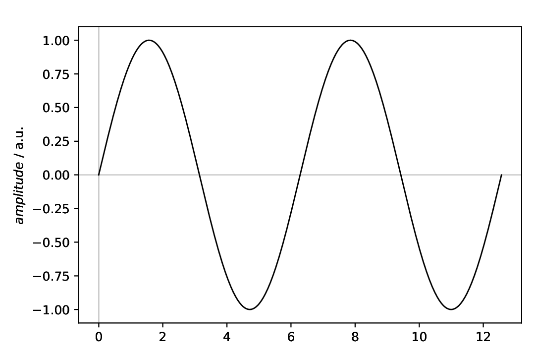
Fig. 3 Sine with standard parameters.
A noisy Gaussian
A model often encountered in spectroscopy is a Gaussian, or bell-shaped curve. There are different Gaussians available as model, namely aspecd.model.Gaussian for the generalised variant, and aspecd.model.NormalisedGaussian for the normalised variant frequently used when describing line shapes of spectral lines.
The task: Create a Gaussian as dataset, add some noise, and plot both, the original and the noisy one afterwards.
 1format:
 2  type: ASpecD recipe
 3  version: '0.3'
 4
 5tasks:
 6  - kind: model
 7    type: Zeros
 8    properties:
 9      parameters:
10        shape: 1001
11        range: [-10, 10]
12    result: dummy
13    comment: >
14      Add some 1/f noise
15
16  - kind: model
17    type: Gaussian
18    from_dataset: dummy
19    properties:
20      parameters:
21        amplitude: 2
22        position: 0.5
23        width: 1.5
24    result: gaussian
25    comment: >
26      Create Gaussian with some parameters set explicitly
27
28  - kind: processing
29    type: Noise
30    properties:
31      parameters:
32        amplitude: 0.3
33    apply_to: gaussian
34    result: noisy-gaussian
35
36  - kind: multiplot
37    type: MultiPlotter1D
38    properties:
39      properties:
40        drawings:
41          - color: "#999999"
42          - color: "#000000"
43      parameters:
44        tight_layout: True
45      filename: model-introduction-gaussian.pdf
46    apply_to:
47      - noisy-gaussian
48      - gaussian
49    comment: >
50      Plot both, noisy and original Gaussian
Comments
The range for the “dummy” dataset has been adjusted to fit a Gaussian with its symmetric, bell-shaped curve.
For the Gaussian, the three possible parameters
amplitude,position, andwidthare set explicitly.For adding the noise, the same applies as for the plot: You need to explicitly provide the model dataset to operate on using the
apply_todirective.When adding the noise, make sure to provide a
resultas well, as we want to plot both, the original and the noisy Gaussian afterwards.For the plot, the sequence you provide the dataset names in the
apply_todirective does matter. Usually, in plots like the one shown here, you would like to have the “model” (noise-free data) shown on top of the experimental data, faked here by adding noise.In the plotter, colours for the individual lines have been set explicitly. Please note that in case of specifying colours in YAML recipes as hexadecimal values, you need to explicitly mark them as string by surrounding them with quotes.
Result
The resulting figure is shown below. While in the recipe, the output format has been set to PDF, for rendering images here they have been converted to PNG.
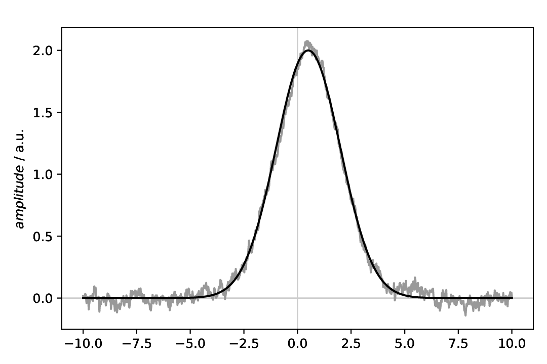
Fig. 4 Gaussian with (coloured, 1/f) noise added, and on top the original Gaussian. Note that due to the random component of the noise, your figure will look different regarding the noise.
Comments
The recipe shown here does not import any data, hence does not have the usual top-level block
datasets, but directly starts with thetasksblock.We need to first define a “dummy” dataset with the correct dimensions. There are two types of models for this task available:
aspecd.model.Zeros(used here) andaspecd.model.Ones.The actual model uses the
from_datasetdirective to obain the dimensions from the “dummy” dataset in the previous step.Plotting requires explicitly mentioning the model dataset using the
apply_todirective.