You're reading the documentation for a development version. For the latest released version, please have a look at v0.12.
UV/Vis spectra normalised to absorption band
Measuring optical absorption (UV/Vis) spectra of samples often results in a series of measurements, and one of the first tasks is to get an overview what has been measured and how the results look like. Furthermore, if we have recorded a series of spectra for different samples, we are often interested in a comparison.
In this particular example, a series of optical absorption spectra for building blocks with varying lengths has been recorded, and we are interested in the shift of the absorption band as a function of the molecules’ length.
To this end, a series of tasks needs to be performed on each dataset:
Import the data (assuming ASCII export)
Normalise to the absorption band, but explicitly not to the entire recorded range, as we will often have more intense side bands we are not interested in for now
Plot all spectra in one axis for graphical display of recorded data
Note
As mentioned previously, using plain ASpecD usually does not help you with a rich data model of your dataset, containing all the relevant metadata. However, in the case shown here, it nicely shows the power of ASpecD on itself. For real and routine analysis of UV/Vis data, you may want to use the UVVisPy package based on the ASpecD framework and available via PyPI.
 1format:
 2  type: ASpecD recipe
 3  version: '0.3'
 4
 5datasets:
 6  - source: tbt.txt
 7    label: TBT
 8    importer: TxtImporter
 9    importer_parameters:
10      skiprows: 2
11      separator: ','
12  - source: cbztbt.txt
13    label: CbzTBT
14    importer: TxtImporter
15    importer_parameters:
16      skiprows: 2
17      separator: ','
18  - source: cbztbtcbz.txt
19    label: CbzTBTCbz
20    importer: TxtImporter
21    importer_parameters:
22      skiprows: 2
23      separator: ','
24  - source: pcdtbt.txt
25    label: PCDTBT
26    importer: TxtImporter
27    importer_parameters:
28      skiprows: 2
29      separator: ','
30
31tasks:
32  - kind: processing
33    type: Normalisation
34    properties:
35      parameters:
36        range: [410, 700]
37        range_unit: axis
38
39  - kind: multiplot
40    type: MultiPlotter1D
41    properties:
42      properties:
43        axes:
44          xlim: [300, 800]
45          xlabel: '$wavelength$ / nm'
46          ylim: [-0.05, 1.4]
47          ylabel: '$normalised\ intensity$'
48      parameters:
49        tight_layout: True
50        show_legend: True
51      filename: uvvis-normalised.pdf
52
Result
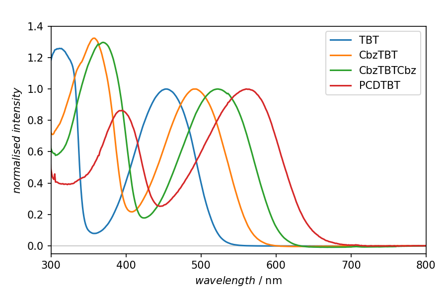
Fig. 1 Result of the plotting step in the recipe shown above. The four spectra presented have been normalised to their low-energy absorption band. A detailed analysis of the data shown here is given in Matt et al. Macromolecules 51:4341–4349, 2018. doi:10.1021/acs.macromol.8b00791.