You're reading the documentation for a development version. For the latest released version, please have a look at v0.10.
Plotting: Spines
Classes used:
Models:
Analysis:
Plotting:
Graphical representation of data and results is one of the most important aspects of presenting scientific results. A good figure is a figure allowing the reader to immediately catch the important aspects, not relying on reading the (nevertheless always important) caption with more description.
Probably, figures are the single most variable and configurable element of scientific data processing and analysis. While for many aspects, conventions have been established, there is much room left for individual adjustments.
Here, we focus on modifying the axes spines: the lines connecting the axis tick marks and noting the boundaries of the data area.
Recipe
Shown below is the entire recipe. As this is quite lengthy, separate parts will be detailed below in the “Results” section.
  1format:
  2  type: ASpecD recipe
  3  version: '0.2'
  4
  5settings:
  6  autosave_plots: False
  7
  8tasks:
  9  - kind: model
 10    type: Zeros
 11    properties:
 12      parameters:
 13        shape: 1001
 14        range: [-3.1415, 4.7124]
 15    result: dummy
 16
 17  - kind: model
 18    type: Sine
 19    from_dataset: dummy
 20    result: model_data
 21    comment: >
 22      Create sine
 23
 24  - kind: singleplot
 25    type: SinglePlotter1D
 26    properties:
 27      properties:
 28        axes:
 29          xlabel: "$position$ / a.u."
 30          spines:
 31            right:
 32              visible: False
 33            top:
 34              visible: False
 35      parameters:
 36        tight_layout: True
 37      filename: plotting-spines-no-top-right.pdf
 38    apply_to:
 39      - model_data
 40    comment: >
 41      Plotter with no spines at top and right
 42
 43  - kind: singleplot
 44    type: SinglePlotter1D
 45    properties:
 46      properties:
 47        axes:
 48          xlabel: "$position$ / a.u."
 49          spines:
 50            left:
 51              bounds: [-1, 1]
 52              position: ["outward", 10]
 53            bottom:
 54              bounds: [-3, 5]
 55              position: ["outward", 10]
 56            right:
 57              visible: False
 58            top:
 59              visible: False
 60      parameters:
 61        tight_layout: True
 62        show_zero_lines: False
 63      filename: plotting-spines-no-top-right-detached.pdf
 64    apply_to:
 65      - model_data
 66    comment: >
 67      Plotter with no spines at top and right and detached spines
 68
 69  - kind: singleplot
 70    type: SinglePlotter1D
 71    properties:
 72      properties:
 73        axes:
 74          xlabel: "$position$ / a.u."
 75          xlabelposition: right
 76          ylabelposition: top
 77          spines:
 78            left:
 79              position: center
 80            bottom:
 81              position: center
 82            right:
 83              visible: False
 84            top:
 85              visible: False
 86      parameters:
 87        tight_layout: True
 88        show_zero_lines: False
 89      filename: plotting-spines-no-top-right-centre.pdf
 90    apply_to:
 91      - model_data
 92    comment: >
 93      Plotter with no spines at top and right and other spines at centre
 94
 95  - kind: singleplot
 96    type: SinglePlotter1D
 97    properties:
 98      properties:
 99        axes:
100          xlabel: "$position$ / a.u."
101          xlabelposition: right
102          ylabelposition: top
103          spines:
104            left:
105              position: zero
106            bottom:
107              position: zero
108            right:
109              visible: False
110            top:
111              visible: False
112      parameters:
113        tight_layout: True
114        show_zero_lines: False
115      filename: plotting-spines-no-top-right-zero.pdf
116    apply_to:
117      - model_data
118    comment: >
119      Plotter with no spines at top and right and other spines at centre
120
121  - kind: singleplot
122    type: SinglePlotter1D
123    properties:
124      properties:
125        axes:
126          xlabel: "$position$ / a.u."
127          xlabelposition: right
128          ylabelposition: top
129          spines:
130            left:
131              position: zero
132              arrow: True
133            bottom:
134              position: zero
135              arrow: True
136            right:
137              visible: False
138            top:
139              visible: False
140      parameters:
141        tight_layout: True
142      filename: plotting-spines-with-arrows.pdf
143    apply_to:
144      - model_data
145    comment: >
146      Plotter with centred spines with arrow
147
148  - kind: singleplot
149    type: SinglePlotter1D
150    properties:
151      properties:
152        axes:
153          xlabel: "$position$ / a.u."
154          xlabelposition: right
155          ylabelposition: top
156          invert:
157            - x
158            - y
159          spines:
160            left:
161              position: zero
162              arrow: True
163            bottom:
164              position: zero
165              arrow: True
166            right:
167              visible: False
168            top:
169              visible: False
170      parameters:
171        tight_layout: True
172      filename: plotting-spines-with-arrows-and-inverted-axes.pdf
173    apply_to:
174      - model_data
175    comment: >
176      Plotter with centred spines with arrow and inverted axes
Results
Examples for the figures created in the recipe are given below. While in the recipe, the output format has been set to PDF, for rendering them here they have been converted to PNG.
As this is a rather lengthy recipe demonstrating different scenarios, the individual cases are shown separately, each with the corresponding section of the recipe.
Only left and bottom spines
The common scenario found often in plots: You don’t want to have the box, but only spines at the left and bottom part of your axes, together with ticks and labels.
24  - kind: singleplot
25    type: SinglePlotter1D
26    properties:
27      properties:
28        axes:
29          xlabel: "$position$ / a.u."
30          spines:
31            right:
32              visible: False
33            top:
34              visible: False
35      parameters:
36        tight_layout: True
37      filename: plotting-spines-no-top-right.pdf
38    apply_to:
39      - model_data
40    comment: >
41      Plotter with no spines at top and right
As you can see, spines have their own key in the axes properties, and there are four spines: left, bottom, right, and top. Here, we simply set the visibility of the right and top spine to False and are done.
The resulting figure is shown below:
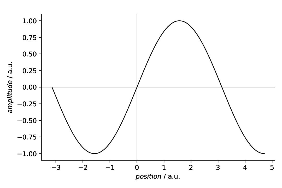
Fig. 15 Plot with only left and bottom spine shown.
Detached spines
Sometimes, you want to “detach” the spines from the data area. Here, it is common to set both, the position as well as the boundaries (bounds) of the spines. Again, we switched off the right and top spines, and positioned the left and bottom spine 10 pt outward of the data area.
43  - kind: singleplot
44    type: SinglePlotter1D
45    properties:
46      properties:
47        axes:
48          xlabel: "$position$ / a.u."
49          spines:
50            left:
51              bounds: [-1, 1]
52              position: ["outward", 10]
53            bottom:
54              bounds: [-3, 5]
55              position: ["outward", 10]
56            right:
57              visible: False
58            top:
59              visible: False
60      parameters:
61        tight_layout: True
62        show_zero_lines: False
63      filename: plotting-spines-no-top-right-detached.pdf
64    apply_to:
65      - model_data
66    comment: >
67      Plotter with no spines at top and right and detached spines
The bounds are in data coordinates, with lower and upper bound, and the position is a list (originally a tuple) with position type and value. For the position, you can choose between “outward” (as used here), “axes”, and “data”. For details, have a look at the documentation of the SpineProperties class. There are two special keywords, “center” and “zero”, that will be detailed below.
The resulting figure is shown below:

Fig. 16 Plot with only left and bottom spines, and both spines detached and restricted in their boundaries. Technically speaking, the bottom spine does not exactly match the data limits, but this is not that unusual for scientific figures.
Positioning spines: centre
Spines need not be positioned left, bottom, right, and top, but can be put to arbitrary positions. There are two special keywords to simplify positioning a bit: “center” will puth the spines to the centre of the coordinate system.
69  - kind: singleplot
70    type: SinglePlotter1D
71    properties:
72      properties:
73        axes:
74          xlabel: "$position$ / a.u."
75          xlabelposition: right
76          ylabelposition: top
77          spines:
78            left:
79              position: center
80            bottom:
81              position: center
82            right:
83              visible: False
84            top:
85              visible: False
86      parameters:
87        tight_layout: True
88        show_zero_lines: False
89      filename: plotting-spines-no-top-right-centre.pdf
90    apply_to:
91      - model_data
92    comment: >
93      Plotter with no spines at top and right and other spines at centre
Whether positioning the spines in the centre is sensible is a decision of your own. This is just to show how the special keyword “center” for the position key works.
The resulting figure is shown below:
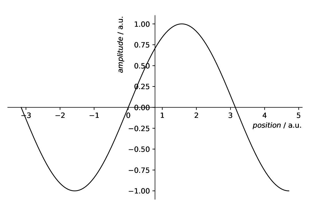
Fig. 17 Plot with only left and bottom spine, and both spines positioned in the centre of the coordinate system, using the special position keyword “center”.
What we have done additionally here is to reposition the axes labels, as having the labels in the centre together with the splines is clearly a bad idea. There are three possibilities to position the axes labels: left, centre, right. For vertical axes, left equals bottom and right equals top.
Positioning spines: origin
Spines need not be positioned left, bottom, right, and top, as mentioned above. They can conveniently be put to the origin of the coordinate system using the special keyword “zero” – and this may make much more sense than positioning them in the centre.
 95  - kind: singleplot
 96    type: SinglePlotter1D
 97    properties:
 98      properties:
 99        axes:
100          xlabel: "$position$ / a.u."
101          xlabelposition: right
102          ylabelposition: top
103          spines:
104            left:
105              position: zero
106            bottom:
107              position: zero
108            right:
109              visible: False
110            top:
111              visible: False
112      parameters:
113        tight_layout: True
114        show_zero_lines: False
115      filename: plotting-spines-no-top-right-zero.pdf
116    apply_to:
117      - model_data
118    comment: >
119      Plotter with no spines at top and right and other spines at centre
The resulting figure is shown below:
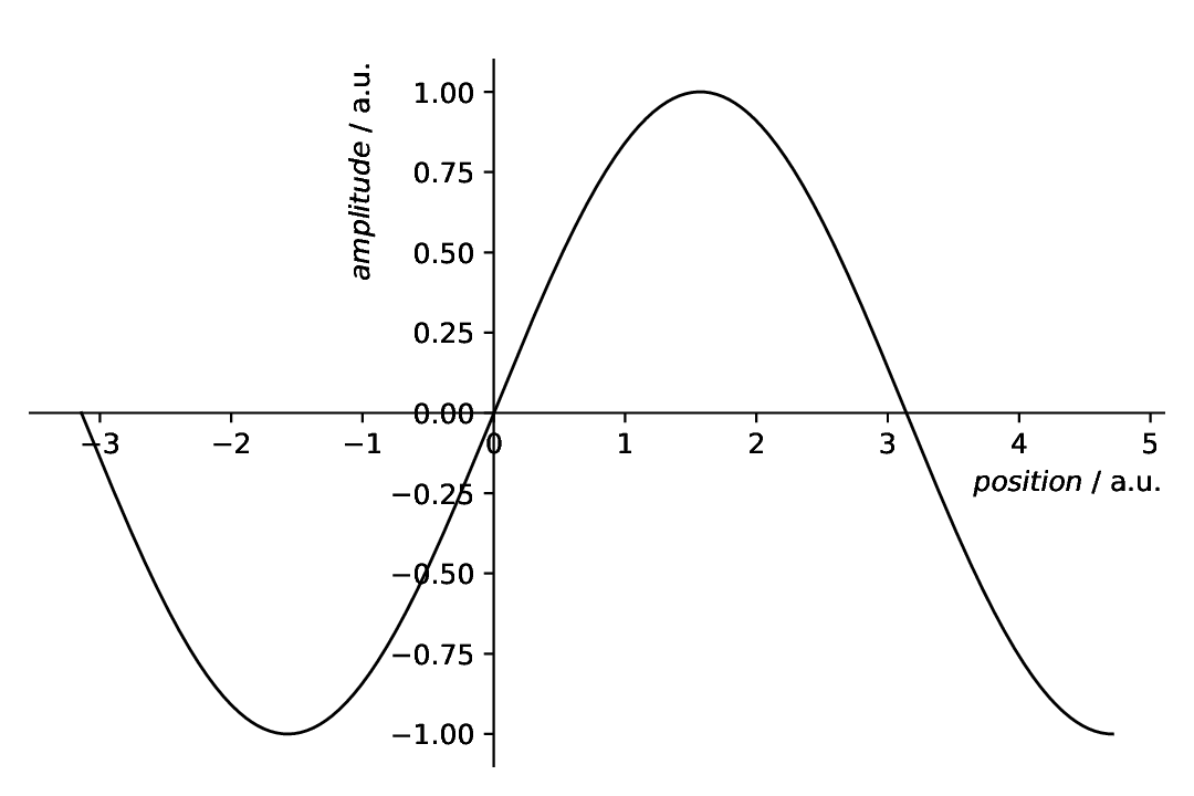
Fig. 18 Plot with only left and bottom spine, and both spines positioned in the origin of the coordinate system, using the special position keyword “zero”.
Again, the axes labels have been repositioned, such as not to clash with the spines. Whether this is necessary in this case depends on the extent of your x and y axes. There are three possibilities to position the axes labels: left, centre, right. For vertical axes, left equals bottom and right equals top.
Spines with arrows
Particularly in case of only showing two spines and having them either centred or positioned in the origin, there may be interest to add arrows to the spines, to create what the Matplotlib documentation calls a “math textbook style plot”. This is possible by setting arrow to True for an individual spine.
121  - kind: singleplot
122    type: SinglePlotter1D
123    properties:
124      properties:
125        axes:
126          xlabel: "$position$ / a.u."
127          xlabelposition: right
128          ylabelposition: top
129          spines:
130            left:
131              position: zero
132              arrow: True
133            bottom:
134              position: zero
135              arrow: True
136            right:
137              visible: False
138            top:
139              visible: False
140      parameters:
141        tight_layout: True
142      filename: plotting-spines-with-arrows.pdf
143    apply_to:
144      - model_data
145    comment: >
146      Plotter with centred spines with arrow
The resulting figure is shown below:
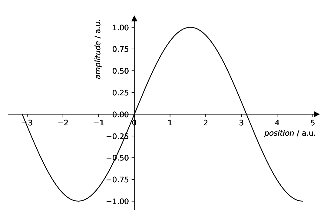
Fig. 19 Plot with only left and bottom spine, both spines positioned in the origin of the coordinate system, using the special position keyword “zero”, and arrows added to the ends of the spines, creating what the Matplotlib documentation calls a “math textbook style plot”.
Note that this is not a default property of the underlying matplotlib.spines.Spine, but adds the arrow heads as additional plots. This functionality is inspired by an example in the Matplotlib documentation: https://matplotlib.org/stable/gallery/spines/centered_spines_with_arrows.html.
Spines with arrows and inverted axes
Having spines with arrow heads is nice, but does it work with inverted axes (as common in FTIR or NMR spectroscopy, to mention just two examples) as well? Yes, of course. ;-)
148  - kind: singleplot
149    type: SinglePlotter1D
150    properties:
151      properties:
152        axes:
153          xlabel: "$position$ / a.u."
154          xlabelposition: right
155          ylabelposition: top
156          invert:
157            - x
158            - y
159          spines:
160            left:
161              position: zero
162              arrow: True
163            bottom:
164              position: zero
165              arrow: True
166            right:
167              visible: False
168            top:
169              visible: False
170      parameters:
171        tight_layout: True
172      filename: plotting-spines-with-arrows-and-inverted-axes.pdf
173    apply_to:
174      - model_data
175    comment: >
176      Plotter with centred spines with arrow and inverted axes
The resulting figure is shown below:
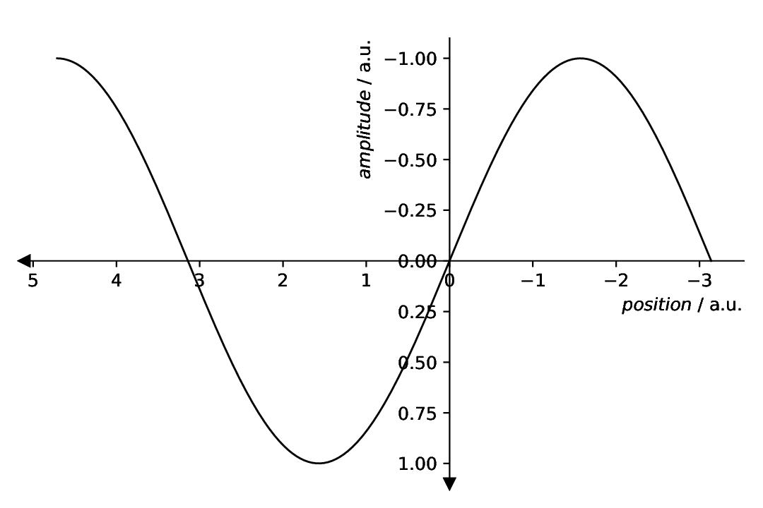
Fig. 20 Plot with only left and bottom spine, both spines positioned in the origin of the coordinate system, using the special position keyword “zero”, both axes inverted using the invert key in the axes properties, and arrows added to the ends of the spines, creating what the Matplotlib documentation calls a “math textbook style plot”.
In this case, the axes labels have been put at the “rear” side of the spines. While typically, you would put the labels close to the arrow heads, in this particular case, that does not make too much sense, at least not for the vertical axis.
Comments
As usual, a model dataset is created at the beginning, to have something to show. Here, a simple sine.
For simplicity, a generic plotter is used, to focus on the spines.