Analysis: Centre of mass
Classes used:
Models:
Analysis:
Processing:
Plotting:
Annotations:
In Physics, the centre of mass of a body is the mass-weighted average of the positions of its mass points. It can be equally applied to an ND dataset, where the mass is related to the intensity value at a given point.
In one dimension, the centre of mass, \(x_s\), can be calculated by:
with the total mass \(M\), i.e. the sum of all point masses:
This can be generalised to arbitrary dimensions, defining the centre of mass as the mass-weighted average of the position vectors \(\vec{r}_i\):
Recipe
Shown below is the entire recipe. As this is quite lengthy, separate parts will be detailed below in the “Results” section.
  1format:
  2  type: ASpecD recipe
  3  version: '0.3'
  4
  5settings:
  6  autosave_plots: False
  7
  8tasks:
  9  - kind: model
 10    type: Zeros
 11    properties:
 12      parameters:
 13        shape: 1001
 14        range: [0, 20]
 15    result: dummy
 16
 17  - kind: model
 18    type: CompositeModel
 19    from_dataset: dummy
 20    properties:
 21      models:
 22        - Lorentzian
 23        - Lorentzian
 24      parameters:
 25        - position: 5
 26          width: 0.8
 27        - position: 8
 28          width: 2
 29    result: model_data
 30
 31  - kind: singleanalysis
 32    type: CentreOfMass
 33    apply_to: model_data
 34    result: centre_of_mass
 35
 36  - kind: singleplot
 37    type: SinglePlotter1D
 38    properties:
 39      properties:
 40        axes:
 41          xlabel: "$position$ / a.u."
 42          xlim: [0, 20]
 43          ylim: [0, 1.35]
 44      parameters:
 45        tight_layout: True
 46      filename: analysis-centre-of-mass-lorentzian.pdf
 47    apply_to:
 48      - model_data
 49    result:
 50      - plot-lorentzian
 51    comment: >
 52      Plotter that gets annotated later
 53
 54  - kind: plotannotation
 55    type: VerticalLine
 56    properties:
 57      parameters:
 58        positions: centre_of_mass
 59      properties:
 60        color: gray
 61        linestyle: dashed
 62    plotter: plot-lorentzian
 63    comment: >
 64      Vertical line marking the centre of mass
 65
 66  - kind: model
 67    type: Ones
 68    properties:
 69      parameters:
 70        shape: [512, 512]
 71        range:
 72          - [200, 350]
 73          - [275, 425]
 74    result: dummy_2D
 75
 76  - kind: singleprocessing
 77    type: Noise
 78    properties:
 79      parameters:
 80        exponent: 0
 81    apply_to: dummy_2D
 82    result: model_data_2D
 83
 84  - kind: singleanalysis
 85    type: CentreOfMass
 86    apply_to: model_data_2D
 87    result: centre_of_mass_2D
 88
 89  - kind: singleplot
 90    type: SinglePlotter2D
 91    properties:
 92      parameters:
 93        tight_layout: True
 94      properties:
 95        axes:
 96          aspect: equal
 97      filename: analysis-centre-of-mass-2D.pdf
 98    apply_to:
 99      - model_data_2D
100    result:
101      - plot-2D
102    comment: >
103      Plotter that gets annotated later
104
105  - kind: plotannotation
106    type: Marker
107    properties:
108      parameters:
109        positions:
110          - centre_of_mass_2D
111        marker: x
112      properties:
113        edgecolor: red
114        size: 12
115    plotter: plot-2D
Results
Examples for the figures created in the recipe are given below. While in the recipe, the output format has been set to PDF, for rendering them here they have been converted to PNG.
As this is a longer recipe demonstrating different scenarios, the individual cases are shown separately, each with the corresponding section of the recipe.
Centre of mass for 1D datasets
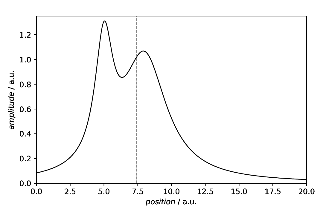
The scenario: We have a curve – in terms of statistics an asymmetric distribution – and want to calculate and display the centre of mass. In spectroscopy, think of an anisotropic line where you would like to get the position of the isotropic peak.
Getting the centre of mass for this asymmetric line is straight-forward and rather unspectacular:
31  - kind: singleanalysis
32    type: CentreOfMass
33    apply_to: model_data
34    result: centre_of_mass
Key here is to save the result to a variable, to be able to use the x coordinate for a plot annotation later on. This is what directly follows in the example recipe: plot the actual data and add a vertical line as plot annotation, using the result from the analysis as position:
36  - kind: singleplot
37    type: SinglePlotter1D
38    properties:
39      properties:
40        axes:
41          xlabel: "$position$ / a.u."
42          xlim: [0, 20]
43          ylim: [0, 1.35]
44      parameters:
45        tight_layout: True
46      filename: analysis-centre-of-mass-lorentzian.pdf
47    apply_to:
48      - model_data
49    result:
50      - plot-lorentzian
51    comment: >
52      Plotter that gets annotated later
53
54  - kind: plotannotation
55    type: VerticalLine
56    properties:
57      parameters:
58        positions: centre_of_mass
59      properties:
60        color: gray
61        linestyle: dashed
62    plotter: plot-lorentzian
63    comment: >
64      Vertical line marking the centre of mass
The resulting figure is shown below:

Fig. 41 Plot of an asymmetric curve with the centre of mass determined using the aspecd.analysis.CentreOfMass analysis step highlighted using a vertical line as plot annotation.
Determining the centre of mass works for arbitrary data in arbitrary dimensions, and even with non-equal spacing of the axes.
Centre of mass for 2D datasets
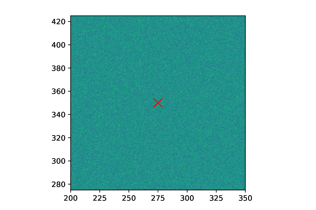
While determining the centre of mass works for arbitrary dimensions, we restrict ourselves here to two dimensions and use the simplest of all models: a 2D array with purely Gaussian noise. In such case, one would expect the centre of mass to be pretty much at the centre of the 2D array, and this is indeed the case, as will be demonstrated in the figure below.
Getting the centre of mass for a 2D dataset is straight-forward and identical to the 1D case:
84  - kind: singleanalysis
85    type: CentreOfMass
86    apply_to: model_data_2D
87    result: centre_of_mass_2D
Key here is again to save the result to a variable, to be able to use the coordinates for a plot annotation later on. Note that in case of 2D data, you will get two coordinates, and generally for nD data, of course n coordinates.
Marking a point in a 2D plot can be done by simply placing a marker at the respective position. For simplicity, we have used a aspecd.annotation.Marker task and placed an “x” at the centre of mass:
 89  - kind: singleplot
 90    type: SinglePlotter2D
 91    properties:
 92      parameters:
 93        tight_layout: True
 94      properties:
 95        axes:
 96          aspect: equal
 97      filename: analysis-centre-of-mass-2D.pdf
 98    apply_to:
 99      - model_data_2D
100    result:
101      - plot-2D
102    comment: >
103      Plotter that gets annotated later
104
105  - kind: plotannotation
106    type: Marker
107    properties:
108      parameters:
109        positions:
110          - centre_of_mass_2D
111        marker: x
112      properties:
113        edgecolor: red
114        size: 12
115    plotter: plot-2D
As we got the coordinates from the analysis step, we can directly use the result in the positions key here. The resulting figure is shown below:

Fig. 42 Plot of a 2D dataset consisting of purely Gaussian noise. As expected, the centre of mass is pretty much at the centre of the dataset.
As the dataset has quadratic shape, we have set the aspect ratio of the plot to equal in this case, in order to not distort the individual data points.
Comments
As usual, model datasets are created, to have something to work with. Here, a CompositeModel comprising of two Lorentizans is used to get an asymmetric curve with an interesting centre of mass. For the 2D case, purely Gaussian noise is created.
For simplicity, generic plotters are used, to focus on the analysis.