You're reading the documentation for a development version. For the latest released version, please have a look at v0.10.
Plot annotations: FillBetween
Classes used:
Models:
Processing:
Plotting:
Annotations:
Graphical representation of data and results is one of the most important aspects of presenting scientific results. A good figure is a figure allowing the reader to immediately catch the important aspects, not relying on reading the (nevertheless always important) caption with more description.
To this end, there is the frequent need to annotate figures, i.e. add additional lines, areas, or even text. This is what can be done with the concrete subclasses of aspecd.annotation.PlotAnnotation.
Here, we focus on filling areas below or between curves that can be used, e.g., to highlight individual components. Suppose you have fitted a spectral line with a series of Lorentzians, and you would like to show the individual components as shaded areas. That’s exactly what aspecd.annotation.FillBetween is designed for.
Recipe
Shown below is the entire recipe. As this is quite lengthy, separate parts will be detailed below in the “Results” section.
  1format:
  2  type: ASpecD recipe
  3  version: '0.2'
  4
  5settings:
  6  autosave_plots: False
  7
  8tasks:
  9  - kind: model
 10    type: Zeros
 11    properties:
 12      parameters:
 13        shape: 1001
 14        range: [0, 20]
 15    result: dummy
 16
 17  - kind: model
 18    type: Lorentzian
 19    from_dataset: dummy
 20    properties:
 21      parameters:
 22        position: 5
 23        width: 0.8
 24    result: lorentzian1
 25
 26  - kind: model
 27    type: Lorentzian
 28    from_dataset: dummy
 29    properties:
 30      parameters:
 31        position: 8
 32        width: 2
 33    result: lorentzian2
 34
 35  - kind: model
 36    type: CompositeModel
 37    from_dataset: dummy
 38    properties:
 39      models:
 40        - Lorentzian
 41        - Lorentzian
 42      parameters:
 43        - position: 5
 44          width: 0.8
 45        - position: 8
 46          width: 2
 47    result: model_data
 48
 49  - kind: multiplot
 50    type: MultiPlotter1D
 51    properties:
 52      properties:
 53        axes:
 54          xlabel: "$position$ / a.u."
 55          xlim: [0, 20]
 56          ylim: [0, 1.45]
 57        drawings:
 58          - linewidth: 1.5
 59            color: black
 60          - linewidth: 1
 61            color: gray
 62          - linewidth: 1
 63            color: gray
 64      parameters:
 65        tight_layout: True
 66      filename: plotting-annotation-fillbetween-no-annotation.pdf
 67    apply_to:
 68      - model_data
 69      - lorentzian1
 70      - lorentzian2
 71    comment: >
 72      Plotter showing just the model.
 73
 74  - kind: multiplot
 75    type: MultiPlotter1D
 76    properties:
 77      properties:
 78        axes:
 79          xlabel: "$position$ / a.u."
 80          xlim: [0, 20]
 81          ylim: [0, 1.45]
 82      parameters:
 83        tight_layout: True
 84      filename: plotting-annotation-fillbetween.pdf
 85    apply_to:
 86      - model_data
 87      - lorentzian1
 88      - lorentzian2
 89    result: plot-with-fillbetween
 90    comment: >
 91      Plotter showing the model and the two coloured surfaces.
 92
 93  - kind: plotannotation
 94    type: FillBetween
 95    properties:
 96      parameters:
 97        data:
 98          - lorentzian1
 99          - lorentzian2
100    plotter: plot-with-fillbetween
101    comment: >
102      Coloured surfaces of the Lorentzians with default properties.
103
104  - kind: multiplot
105    type: MultiPlotter1D
106    properties:
107      properties:
108        axes:
109          xlabel: "$position$ / a.u."
110          xlim: [0, 20]
111          ylim: [0, 1.45]
112      parameters:
113        tight_layout: True
114      filename: plotting-annotation-fillbetween-separate.pdf
115    apply_to:
116      - model_data
117      - lorentzian1
118      - lorentzian2
119    result: plot-with-fillbetween-separate
120    comment: >
121      Plotter showing the model and the two coloured surfaces separately styled.
122
123  - kind: plotannotation
124    type: FillBetween
125    properties:
126      parameters:
127        data:
128          - lorentzian1
129      properties:
130        facecolor: orange
131        alpha: 0.3
132    plotter: plot-with-fillbetween-separate
133    result: fillbetween-lorentzian1
134    comment: >
135      Coloured surfaces of the first Lorentzian.
136
137  - kind: plotannotation
138    type: FillBetween
139    properties:
140      parameters:
141        data:
142          - lorentzian2
143      properties:
144        facecolor: green
145        alpha: 0.3
146    plotter: plot-with-fillbetween-separate
147    result: fillbetween-lorentzian2
148    comment: >
149      Coloured surfaces of the second Lorentzian.
150
151  - kind: singleplot
152    type: SinglePlotter1D
153    properties:
154      properties:
155        axes:
156          xlabel: "$position$ / a.u."
157          xlim: [0, 20]
158          ylim: [0, 1.45]
159      parameters:
160        tight_layout: True
161      filename: plotting-annotation-fillbetween-singleplot.pdf
162    apply_to:
163      - model_data
164    annotations:
165      - fillbetween-lorentzian1
166      - fillbetween-lorentzian2
167    comment: >
168      Plotter showing the model and the two coloured surfaces marking the components.
169
170  - kind: model
171    type: Polynomial
172    from_dataset: dummy
173    properties:
174      parameters:
175        coefficients: [0.1, 0.01]
176    result: baseline
177
178  - kind: processing
179    type: DatasetAlgebra
180    properties:
181      parameters:
182        kind: add
183        dataset: baseline
184    apply_to: model_data
185    result: model_data_with_baseline
186
187  - kind: processing
188    type: DatasetAlgebra
189    properties:
190      parameters:
191        kind: add
192        dataset: baseline
193    apply_to: lorentzian1
194    result: lorentzian1_with_baseline
195
196  - kind: processing
197    type: DatasetAlgebra
198    properties:
199      parameters:
200        kind: add
201        dataset: baseline
202    apply_to: lorentzian2
203    result: lorentzian2_with_baseline
204
205  - kind: multiplot
206    type: MultiPlotter1D
207    properties:
208      properties:
209        axes:
210          xlabel: "$position$ / a.u."
211          xlim: [0, 20]
212        drawings:
213          - color: black
214            linewidth: 1.5
215          - color: gray
216            linewidth: 1
217      parameters:
218        tight_layout: True
219      filename: plotting-annotation-fillbetween-baseline.pdf
220    apply_to:
221      - model_data_with_baseline
222      - baseline
223
224  - kind: plotannotation
225    type: FillBetween
226    properties:
227      parameters:
228        data:
229          - lorentzian1_with_baseline
230        second:
231          - baseline
232      properties:
233        facecolor: orange
234        alpha: 0.3
235    result: fillbetween-lorentzian1_with_baseline
236    comment: >
237      Coloured surfaces of the first Lorentzian.
238
239  - kind: plotannotation
240    type: FillBetween
241    properties:
242      parameters:
243        data:
244          - lorentzian2_with_baseline
245        second:
246          - baseline
247      properties:
248        facecolor: green
249        alpha: 0.3
250    result: fillbetween-lorentzian2_with_baseline
251    comment: >
252      Coloured surfaces of the second Lorentzian.
253
254  - kind: singleplot
255    type: SinglePlotter1D
256    properties:
257      properties:
258        axes:
259          xlabel: "$position$ / a.u."
260          xlim: [0, 20]
261      parameters:
262        tight_layout: True
263      filename: plotting-annotation-fillbetween-with-baseline.pdf
264    apply_to:
265      - model_data_with_baseline
266    annotations:
267      - fillbetween-lorentzian1_with_baseline
268      - fillbetween-lorentzian2_with_baseline
269    comment: >
270      Plotter showing the model and the two coloured surfaces
271      marking the components, but limited by the baseline.
Results
Examples for the figures created in the recipe are given below. While in the recipe, the output format has been set to PDF, for rendering them here they have been converted to PNG.
As this is a rather lengthy recipe demonstrating different scenarios, the individual cases are shown separately, each with the corresponding section of the recipe.
Setting the scene
The scenario: We have a curve comprising of two overlapping Lorentzians and want to highlight the individual components. Here, we just plot the data and the individual components.
49      parameters:
50        tight_layout: True
51      filename: plotting-annotation-marker-default.pdf
52    apply_to:
53      - model_data
54    result:
55      - plot-with-marker
56    comment: >
57      Plotter that gets annotated later
58
59  - kind: plotannotation
60    type: Marker
61    properties:
62      parameters:
63        xpositions: peaks
64        ypositions: 1.38
65        marker: "*"
66    plotter: plot-with-marker
67    comment: >
68      Star-shaped markers with default styling to highlight the peaks.
69
70  - kind: singleplot
71    type: SinglePlotter1D
72    properties:
The resulting figure is shown below:
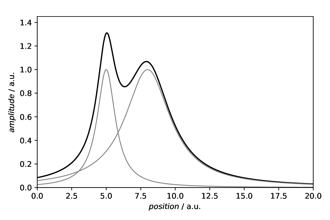
Fig. 35 Plot showing the composite model consisting of two Lorentzians together with the individual components. This is a typical scenario where one would like to add a shading below the curves of the individual components.
FillBetween with default settings
The scenario is as described above: We have a curve comprising of two overlapping Lorentzians and want to highlight the individual components. To fill the area below the curves of the individual components, we can use a aspecd.annotation.FillBetween annotation.
 74        axes:
 75          xlabel: "$position$ / a.u."
 76          xlim: [0, 20]
 77          ylim: [0, 1.45]
 78      parameters:
 79        tight_layout: True
 80      filename: plotting-annotation-marker-styled.pdf
 81    apply_to:
 82      - model_data
 83    result:
 84      - plot-with-styled-marker
 85    comment: >
 86      Plotter that gets annotated later
 87
 88  - kind: plotannotation
 89    type: Marker
 90    properties:
 91      parameters:
 92        xpositions: peaks
 93        ypositions: 1.38
 94        marker: "h"
 95      properties:
 96        edgecolor: red
 97        edgewidth: 2
 98        facecolor: blue
 99        facecoloralt: green
100        size: 16
101        fillstyle: top
102        alpha: 0.8
The resulting figure is shown below:
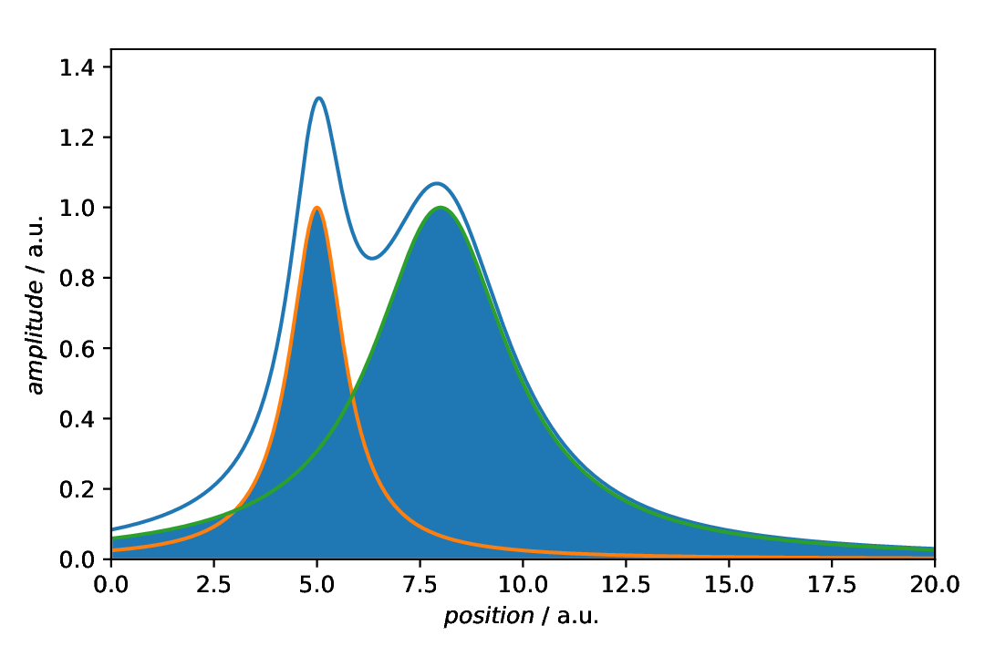
Fig. 36 Plot with shading of the individual components as annotation. Note that the individual components are plotted explicitly as well, using a aspecd.plotting.MultiPlotter1D.
The default settings are most probably not exactly what we usually want to have. First of all, individual components should often been marked with different colours, and adding a bit of transparency may help as well. Off we go.
Individual annotations with styling
In the example above, we have shown the default styling of the aspecd.annotation.FillBetween annotation. As this is not quite what we usually would like to see, here, we apply some styling. For details of the parameters you can set, have a look at aspecd.plotting.PatchProperties.
104    comment: >
105      Styled markers demonstrating some of the styling possibilities.
106
107  - kind: singleanalysis
108    type: PeakFinding
109    properties:
110      parameters:
111        return_intensities: True
112    apply_to: model_data
113    result: peaks_xy
114
115  - kind: singleplot
116    type: SinglePlotter1D
117    properties:
118      properties:
119        axes:
120          xlabel: "$position$ / a.u."
121          xlim: [0, 20]
122          ylim: [0, 1.45]
123      parameters:
124        tight_layout: True
125      filename: plotting-annotation-marker-peaks.pdf
126    apply_to:
127      - model_data
128    result:
129      - plot-with-marker-peaks
130    comment: >
131      Plotter that gets annotated later
132
133  - kind: plotannotation
134    type: Marker
135    properties:
136      parameters:
137        positions: peaks_xy
138        marker: "*"
139    plotter: plot-with-marker-peaks
140    comment: >
141      Star-shaped markers with default styling placed on peaks.
142
143  - kind: singleplot
144    type: SinglePlotter1D
145    properties:
146      properties:
147        axes:
148          xlabel: "$position$ / a.u."
149          xlim: [0, 20]
The resulting figure is shown below:
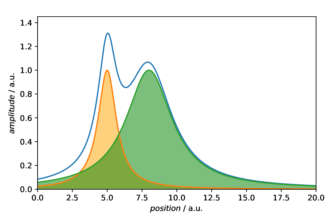
Fig. 37 Plot with both components styled individually. Here, we applied a colour (note the difference between facecolor and edgecolor for this type of annotation) and some transparency.
Individual annotations in a SinglePlotter
Quite similar to the situation above, we need not use a aspecd.plotting.MultiPlotter to show the individual components, as the annotation would be sufficient. Note that we stored the annotations for the individual lines declared above using the result key, so that we can reuse them here.
151      parameters:
152        tight_layout: True
153      filename: plotting-annotation-marker-peaks-yoffset.pdf
154    apply_to:
155      - model_data
156    result:
157      - plot-with-marker-peaks-yoffset
158    comment: >
159      Plotter that gets annotated later
160
161  - kind: plotannotation
162    type: Marker
163    properties:
164      parameters:
165        positions: peaks_xy
166        yoffset: 0.05
167        marker: "*"
168    plotter: plot-with-marker-peaks-yoffset
The resulting figure is shown below:
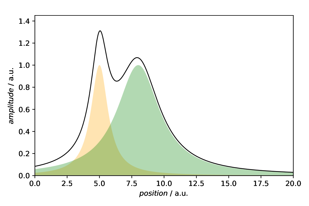
Fig. 38 Plot showing only the line of the composite model, annotated with the shaded areas of the indivual components.
Data with baseline
By default, and if not providing a second line, the patch extends from zero to the data points given by the actual data of the curve. While you could set a scalar value different from zero, more often you will encounter baselines, at least in spectroscopy and in real life. Here, we first (re)create the same data as above, but this time with a baseline added. To add the baseline to both, the model data and the individual components, we use the aspecd.processing.DatasetAlgebra processing step. Afterwards, the data with baseline are plotted together with the baseline.
170      Star-shaped markers with default styling placed on peaks, vertically offset.
171
172  - kind: singleplot
173    type: SinglePlotter1D
174    properties:
175      properties:
176        axes:
177          xlabel: "$position$ / a.u."
178          xlim: [0, 20]
179          ylim: [0, 1.45]
180      parameters:
181        tight_layout: True
182      filename: plotting-annotation-marker-by-name.pdf
183    apply_to:
184      - model_data
185    result:
186      - plot-with-marker-by-name
187    comment: >
188      Plotter that gets annotated later
189
190  - kind: plotannotation
191    type: Marker
192    properties:
193      parameters:
194        positions: peaks_xy
195        yoffset: 0.005
196        marker: "caretdown"
197      properties:
198        edgewidth: 0
199    plotter: plot-with-marker-by-name
200    comment: >
201      Markers with default styling identified by their name.
202
203  - kind: singleplot
204    type: SinglePlotter1D
205    properties:
206      properties:
207        axes:
208          xlabel: "$position$ / a.u."
209          xlim: [0, 20]
210          ylim: [0, 1.45]
211      parameters:
212        tight_layout: True
213      filename: plotting-annotation-marker-mathtext.pdf
214    apply_to:
215      - model_data
216    result:
217      - plot-with-marker-mathtext
218    comment: >
219      Plotter that gets annotated later
220
221  - kind: plotannotation
222    type: Marker
The resulting figure is shown below:
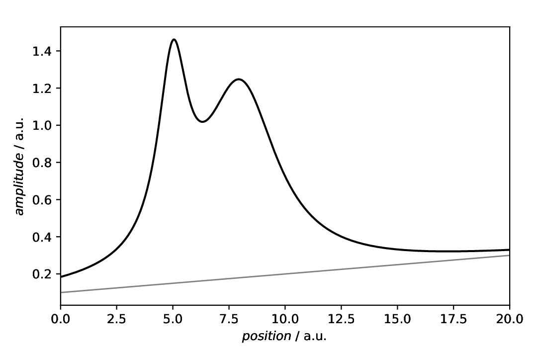
Fig. 39 Data with a baseline added, together with the baseline. A bit of styling is applied here, to show that the baseline is just an addition, not the actual data of interest.
Filling between two curves
Having data with a baseline, this is finally a sensible real-world situation where you may want to provide a second dataset as boundary for the patch. Of course, other typical scenarios are marking the confidence interval of a fit, where you have the lower and upper boundaries as dataset.
224      parameters:
225        positions: peaks_xy
226        yoffset: 0.05
227        marker: $\mathcal{A}$
228      properties:
229        size: 14
230        edgewidth: 0
231        facecolor: orange
232    plotter: plot-with-marker-mathtext
233    comment: >
234      Markers with default styling using MathText (no LaTeX install needed).
235
236      Note that in this case, you cannot have question marks surrounding the
237      marker string, as otherwise, YAML is unhappy.
238
239  - kind: singleplot
240    type: SinglePlotter1D
241    properties:
242      properties:
243        axes:
244          xlabel: "$position$ / a.u."
245          xlim: [0, 20]
246          ylim: [0, 1.45]
247      parameters:
248        tight_layout: True
249      filename: plotting-annotation-marker-unicode.pdf
250    apply_to:
251      - model_data
252    result:
253      - plot-with-marker-unicode
254    comment: >
255      Plotter that gets annotated later
256
257  - kind: plotannotation
258    type: Marker
259    properties:
260      parameters:
261        positions: peaks_xy
262        yoffset: 0.06
263        marker: "$\u266B$"
264      properties:
265        size: 14
266        edgewidth: 0
267        facecolor: blue
268    plotter: plot-with-marker-unicode
269    comment: >
270      Markers with default styling using Unicode (there is music in the peaks).
271
272      Note that in this case, you need to have question marks surrounding the
The resulting figure is shown below:
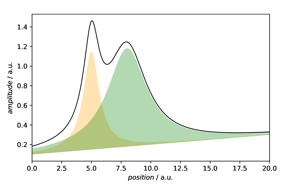
Fig. 40 Data with baseline together with the individual components, but respecting the baseline as (in this case lower) boundary of the fill patch.
Comments
As usual, a model dataset is created at the beginning, to have something to show. Here, a CompositeModel comprising of two Lorentizans is used to get two peaks that can be labelled.
Furthermore, the individual Lorentzians are created as well.
For simplicity, generic plotters are used, to focus on the annotations.
The sequence of defining plot and annotation(s) does not matter. You only need to provide the
resultkey with a unique name for whichever task you define first, to refer to it in the later task(s).