You're reading the documentation for a development version. For the latest released version, please have a look at v0.10.
Plot annotations: Marker (symbols)
Classes used:
Models:
Analysis:
Plotting:
Annotations:
Graphical representation of data and results is one of the most important aspects of presenting scientific results. A good figure is a figure allowing the reader to immediately catch the important aspects, not relying on reading the (nevertheless always important) caption with more description.
To this end, there is the frequent need to annotate figures, i.e. add additional lines, areas, or even text. This is what can be done with the concrete subclasses of aspecd.annotation.PlotAnnotation.
Here, we focus on simple markers (symbols) added to a plot that are often used to label peaks.
Recipe
Shown below is the entire recipe. As this is quite lengthy, separate parts will be detailed below in the “Results” section.
  1format:
  2  type: ASpecD recipe
  3  version: '0.2'
  4
  5settings:
  6  autosave_plots: False
  7
  8tasks:
  9  - kind: model
 10    type: Zeros
 11    properties:
 12      parameters:
 13        shape: 1001
 14        range: [0, 20]
 15    result: dummy
 16
 17  - kind: model
 18    type: CompositeModel
 19    from_dataset: dummy
 20    properties:
 21      models:
 22        - Lorentzian
 23        - Lorentzian
 24      parameters:
 25        - position: 5
 26          width: 0.8
 27        - position: 8
 28          width: 2
 29    result: model_data
 30
 31  - kind: singleanalysis
 32    type: PeakFinding
 33    apply_to: model_data
 34    result: peaks
 35
 36  - kind: singleplot
 37    type: SinglePlotter1D
 38    properties:
 39      properties:
 40        axes:
 41          xlabel: "$position$ / a.u."
 42          xlim: [0, 20]
 43          ylim: [0, 1.45]
 44        grid:
 45          show: True
 46          axis: x
 47          lines:
 48            linestyle: ":"
 49      parameters:
 50        tight_layout: True
 51      filename: plotting-annotation-marker-default.pdf
 52    apply_to:
 53      - model_data
 54    result:
 55      - plot-with-marker
 56    comment: >
 57      Plotter that gets annotated later
 58
 59  - kind: plotannotation
 60    type: Marker
 61    properties:
 62      parameters:
 63        xpositions: peaks
 64        ypositions: 1.38
 65        marker: "*"
 66    plotter: plot-with-marker
 67    comment: >
 68      Star-shaped markers with default styling to highlight the peaks.
 69
 70  - kind: singleplot
 71    type: SinglePlotter1D
 72    properties:
 73      properties:
 74        axes:
 75          xlabel: "$position$ / a.u."
 76          xlim: [0, 20]
 77          ylim: [0, 1.45]
 78      parameters:
 79        tight_layout: True
 80      filename: plotting-annotation-marker-styled.pdf
 81    apply_to:
 82      - model_data
 83    result:
 84      - plot-with-styled-marker
 85    comment: >
 86      Plotter that gets annotated later
 87
 88  - kind: plotannotation
 89    type: Marker
 90    properties:
 91      parameters:
 92        xpositions: peaks
 93        ypositions: 1.38
 94        marker: "h"
 95      properties:
 96        edgecolor: red
 97        edgewidth: 2
 98        facecolor: blue
 99        facecoloralt: green
100        size: 16
101        fillstyle: top
102        alpha: 0.8
103    plotter: plot-with-styled-marker
104    comment: >
105      Styled markers demonstrating some of the styling possibilities.
106
107  - kind: singleanalysis
108    type: PeakFinding
109    properties:
110      parameters:
111        return_intensities: True
112    apply_to: model_data
113    result: peaks_xy
114
115  - kind: singleplot
116    type: SinglePlotter1D
117    properties:
118      properties:
119        axes:
120          xlabel: "$position$ / a.u."
121          xlim: [0, 20]
122          ylim: [0, 1.45]
123      parameters:
124        tight_layout: True
125      filename: plotting-annotation-marker-peaks.pdf
126    apply_to:
127      - model_data
128    result:
129      - plot-with-marker-peaks
130    comment: >
131      Plotter that gets annotated later
132
133  - kind: plotannotation
134    type: Marker
135    properties:
136      parameters:
137        positions: peaks_xy
138        marker: "*"
139    plotter: plot-with-marker-peaks
140    comment: >
141      Star-shaped markers with default styling placed on peaks.
142
143  - kind: singleplot
144    type: SinglePlotter1D
145    properties:
146      properties:
147        axes:
148          xlabel: "$position$ / a.u."
149          xlim: [0, 20]
150          ylim: [0, 1.45]
151      parameters:
152        tight_layout: True
153      filename: plotting-annotation-marker-peaks-yoffset.pdf
154    apply_to:
155      - model_data
156    result:
157      - plot-with-marker-peaks-yoffset
158    comment: >
159      Plotter that gets annotated later
160
161  - kind: plotannotation
162    type: Marker
163    properties:
164      parameters:
165        positions: peaks_xy
166        yoffset: 0.05
167        marker: "*"
168    plotter: plot-with-marker-peaks-yoffset
169    comment: >
170      Star-shaped markers with default styling placed on peaks, vertically offset.
171
172  - kind: singleplot
173    type: SinglePlotter1D
174    properties:
175      properties:
176        axes:
177          xlabel: "$position$ / a.u."
178          xlim: [0, 20]
179          ylim: [0, 1.45]
180      parameters:
181        tight_layout: True
182      filename: plotting-annotation-marker-by-name.pdf
183    apply_to:
184      - model_data
185    result:
186      - plot-with-marker-by-name
187    comment: >
188      Plotter that gets annotated later
189
190  - kind: plotannotation
191    type: Marker
192    properties:
193      parameters:
194        positions: peaks_xy
195        yoffset: 0.005
196        marker: "caretdown"
197      properties:
198        edgewidth: 0
199    plotter: plot-with-marker-by-name
200    comment: >
201      Markers with default styling identified by their name.
202
203  - kind: singleplot
204    type: SinglePlotter1D
205    properties:
206      properties:
207        axes:
208          xlabel: "$position$ / a.u."
209          xlim: [0, 20]
210          ylim: [0, 1.45]
211      parameters:
212        tight_layout: True
213      filename: plotting-annotation-marker-mathtext.pdf
214    apply_to:
215      - model_data
216    result:
217      - plot-with-marker-mathtext
218    comment: >
219      Plotter that gets annotated later
220
221  - kind: plotannotation
222    type: Marker
223    properties:
224      parameters:
225        positions: peaks_xy
226        yoffset: 0.05
227        marker: $\mathcal{A}$
228      properties:
229        size: 14
230        edgewidth: 0
231        facecolor: orange
232    plotter: plot-with-marker-mathtext
233    comment: >
234      Markers with default styling using MathText (no LaTeX install needed).
235
236      Note that in this case, you cannot have question marks surrounding the
237      marker string, as otherwise, YAML is unhappy.
238
239  - kind: singleplot
240    type: SinglePlotter1D
241    properties:
242      properties:
243        axes:
244          xlabel: "$position$ / a.u."
245          xlim: [0, 20]
246          ylim: [0, 1.45]
247      parameters:
248        tight_layout: True
249      filename: plotting-annotation-marker-unicode.pdf
250    apply_to:
251      - model_data
252    result:
253      - plot-with-marker-unicode
254    comment: >
255      Plotter that gets annotated later
256
257  - kind: plotannotation
258    type: Marker
259    properties:
260      parameters:
261        positions: peaks_xy
262        yoffset: 0.06
263        marker: "$\u266B$"
264      properties:
265        size: 14
266        edgewidth: 0
267        facecolor: blue
268    plotter: plot-with-marker-unicode
269    comment: >
270      Markers with default styling using Unicode (there is music in the peaks).
271
272      Note that in this case, you need to have question marks surrounding the
273      marker string, as otherwise, YAML is unhappy.
Results
Examples for the figures created in the recipe are given below. While in the recipe, the output format has been set to PDF, for rendering them here they have been converted to PNG.
As this is a rather lengthy recipe demonstrating different scenarios, the individual cases are shown separately, each with the corresponding section of the recipe.
Simple marker
The scenario: We have a curve comprising of two overlapping Lorentzians and want to highlight the peaks. Using the aspecd.analysis.PeakFinding analysis step allows us to place the labels at the correct x positions.
Here, we first plot the data, and afterwards annotate the plot with an annotation. This is why the plot task as a result set with its result key that is referred to in the annotation task with the plotter key.
36  - kind: singleplot
37    type: SinglePlotter1D
38    properties:
39      properties:
40        axes:
41          xlabel: "$position$ / a.u."
42          xlim: [0, 20]
43          ylim: [0, 1.45]
44        grid:
45          show: True
46          axis: x
47          lines:
48            linestyle: ":"
49      parameters:
50        tight_layout: True
51      filename: plotting-annotation-marker-default.pdf
52    apply_to:
53      - model_data
54    result:
55      - plot-with-marker
56    comment: >
57      Plotter that gets annotated later
58
59  - kind: plotannotation
60    type: Marker
61    properties:
62      parameters:
63        xpositions: peaks
64        ypositions: 1.38
65        marker: "*"
66    plotter: plot-with-marker
67    comment: >
68      Star-shaped markers with default styling to highlight the peaks.
As we got the x positions for our text labels from the analysis step (PeakFinding), we use the xpositions``and ``ypositions keys here, rather than the simple positions key. Furthermore, as we want to have both labels appear with the same y position, we can provide a scalar here for the key ypositions. marker is a single identifier for the marker, and we used the shorthand for the star here.
The appearance of the markers can be controlled in quite some detail. For the styling available, see the documentation of the aspecd.plotting.MarkerProperties class - and use sparingly in scientific context. After all, it is science, not pop art.
The resulting figure is shown below:
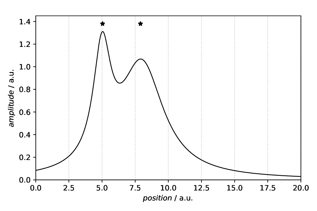
Fig. 28 Plot with two stars marking for the peak positions. Here, the default settings (colours and size) have been used. Note that in this case, the plot(ter) has been defined first, with a result key for later reference, and the annotation afterwards, referring to the plotter using the plotter key.
To demonstrate that the markers are indeed horizontally centred about the peaks, a grid (vertical dotted lines) has been added as guide for the eye of the reader in this case.
Styling the markers
The scenario is the same as above: We have a curve comprising of two overlapping Lorentzians and want to highlight the peaks. Using the aspecd.analysis.PeakFinding analysis step allows us to place the labels at the correct x positions.
Although not sensible in this particular case, this time the markers are styled extensively, just to show what is generally possible. For further details, refer to the documentation of the aspecd.plotting.MarkerProperties class.
 70  - kind: singleplot
 71    type: SinglePlotter1D
 72    properties:
 73      properties:
 74        axes:
 75          xlabel: "$position$ / a.u."
 76          xlim: [0, 20]
 77          ylim: [0, 1.45]
 78      parameters:
 79        tight_layout: True
 80      filename: plotting-annotation-marker-styled.pdf
 81    apply_to:
 82      - model_data
 83    result:
 84      - plot-with-styled-marker
 85    comment: >
 86      Plotter that gets annotated later
 87
 88  - kind: plotannotation
 89    type: Marker
 90    properties:
 91      parameters:
 92        xpositions: peaks
 93        ypositions: 1.38
 94        marker: "h"
 95      properties:
 96        edgecolor: red
 97        edgewidth: 2
 98        facecolor: blue
 99        facecoloralt: green
100        size: 16
101        fillstyle: top
102        alpha: 0.8
103    plotter: plot-with-styled-marker
104    comment: >
105      Styled markers demonstrating some of the styling possibilities.
As we got the x positions for our text labels from the analysis step (PeakFinding), we use the xpositions``and ``ypositions keys here, rather than the simple positions key. In this case, we want to have the labels appear close to the actual line, hence with different y positions. Therefore, the ypositions key contains a list. As marker, we have used h here, a shorthand for a hexagon. Note that there is a variant H as well, with the hexagon standing on an edge rather than a tip, as in this case.
The appearance of the marker can be controlled in quite some detail. For the styling available, see the documentation of the aspecd.plotting.MarkerProperties class - and use sparingly in scientific context. After all, it is science, not pop art.
The resulting figure is shown below:
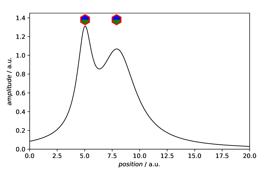
Fig. 29 Plot with two markers for the peak positions as annotation. The markers are heavily styled, and a larger symbol used to show all the details.
Markers placed at the peaks
In the example above, we have shown how to automatically position the markers at the peak positions in the x direction, but still have positioned the annotations in the y direction manually. How about getting both, x and y position of the peaks automatically?
This is possible by using a new feature of the aspecd.analysis.PeakFinding class, namely to explicitly return the intensities as well. Thus, you get a two-dimensional (two-column) numpy array with the peak positions (x values) in the first and the peak intensities (y values) in the second column. This can nicely be used to directly feed it into the positions key of the annotation;
107  - kind: singleanalysis
108    type: PeakFinding
109    properties:
110      parameters:
111        return_intensities: True
112    apply_to: model_data
113    result: peaks_xy
114
115  - kind: singleplot
116    type: SinglePlotter1D
117    properties:
118      properties:
119        axes:
120          xlabel: "$position$ / a.u."
121          xlim: [0, 20]
122          ylim: [0, 1.45]
123      parameters:
124        tight_layout: True
125      filename: plotting-annotation-marker-peaks.pdf
126    apply_to:
127      - model_data
128    result:
129      - plot-with-marker-peaks
130    comment: >
131      Plotter that gets annotated later
132
133  - kind: plotannotation
134    type: Marker
135    properties:
136      parameters:
137        positions: peaks_xy
138        marker: "*"
139    plotter: plot-with-marker-peaks
140    comment: >
141      Star-shaped markers with default styling placed on peaks.
The resulting figure is shown below:

Fig. 30 Plot with two markers for the peak positions as annotation. Instead of only providing the xpositions by the result of the PeakFinding analysis step, we got both, x and y positions, and thus used the positions key instead.
While it is clearly convenient to place the markers automatically in both, x and y direction, having the markers directly on the line is usually not satisfying. How about providing a (small) offset? We’ve got you covered…
Markers placed at the peaks with vertical offset
In the example above, we have shown how to automatically position the markers at the peak positions in x and y direction, but the result was not entirely satisfying, as the marker usually sits on the line. How about having a small vertical offset?
143  - kind: singleplot
144    type: SinglePlotter1D
145    properties:
146      properties:
147        axes:
148          xlabel: "$position$ / a.u."
149          xlim: [0, 20]
150          ylim: [0, 1.45]
151      parameters:
152        tight_layout: True
153      filename: plotting-annotation-marker-peaks-yoffset.pdf
154    apply_to:
155      - model_data
156    result:
157      - plot-with-marker-peaks-yoffset
158    comment: >
159      Plotter that gets annotated later
160
161  - kind: plotannotation
162    type: Marker
163    properties:
164      parameters:
165        positions: peaks_xy
166        yoffset: 0.05
167        marker: "*"
168    plotter: plot-with-marker-peaks-yoffset
169    comment: >
170      Star-shaped markers with default styling placed on peaks, vertically offset.
The resulting figure is shown below:
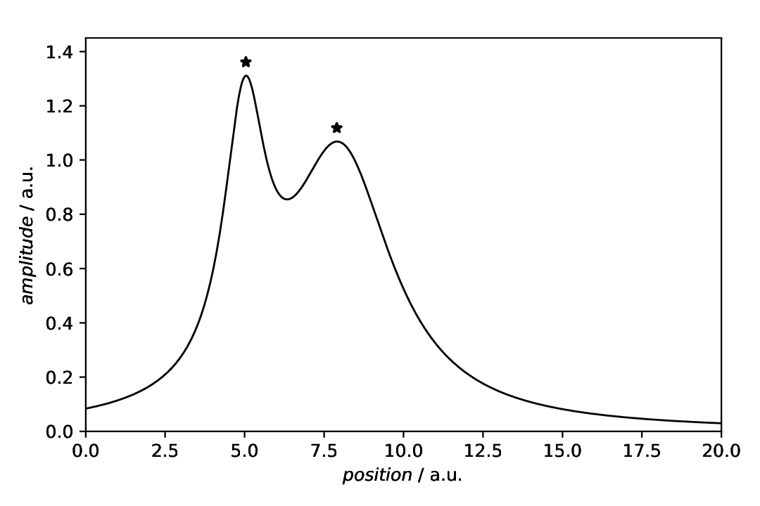
Fig. 31 Plot with two markers for the peak positions as annotation. Instead of only providing the xpositions by the result of the PeakFinding analysis step, we got both, x and y positions, and thus used the positions key instead. Furthermore, using the yoffset key, we placed the markers slightly above the actual line.
Markers identified by name
There is a larger number of pre-defined markers available, and you can of course look up the symbols. However, there is an alternative: use readable names instead. For details, have a look at the documentation of the aspecd.plotting.MarkerProperties.marker attribute.
172  - kind: singleplot
173    type: SinglePlotter1D
174    properties:
175      properties:
176        axes:
177          xlabel: "$position$ / a.u."
178          xlim: [0, 20]
179          ylim: [0, 1.45]
180      parameters:
181        tight_layout: True
182      filename: plotting-annotation-marker-by-name.pdf
183    apply_to:
184      - model_data
185    result:
186      - plot-with-marker-by-name
187    comment: >
188      Plotter that gets annotated later
189
190  - kind: plotannotation
191    type: Marker
192    properties:
193      parameters:
194        positions: peaks_xy
195        yoffset: 0.005
196        marker: "caretdown"
197      properties:
198        edgewidth: 0
199    plotter: plot-with-marker-by-name
200    comment: >
201      Markers with default styling identified by their name.
The resulting figure is shown below:

Fig. 32 Plot with markers identified by their name. Note that in this case, we added a very small vertical offset and set the edgewidth to zero, as depending on the type of marker, having finite edges looks a bit ugly.
Markers using MathText
Although there is a larger number of pre-defined markers available, you can make use of the MathText feature of Matplotlib, even without LaTeX being installed, and put a huge variety of markers to your plots, using LaTeX syntax.
203  - kind: singleplot
204    type: SinglePlotter1D
205    properties:
206      properties:
207        axes:
208          xlabel: "$position$ / a.u."
209          xlim: [0, 20]
210          ylim: [0, 1.45]
211      parameters:
212        tight_layout: True
213      filename: plotting-annotation-marker-mathtext.pdf
214    apply_to:
215      - model_data
216    result:
217      - plot-with-marker-mathtext
218    comment: >
219      Plotter that gets annotated later
220
221  - kind: plotannotation
222    type: Marker
223    properties:
224      parameters:
225        positions: peaks_xy
226        yoffset: 0.05
227        marker: $\mathcal{A}$
228      properties:
229        size: 14
230        edgewidth: 0
231        facecolor: orange
232    plotter: plot-with-marker-mathtext
233    comment: >
234      Markers with default styling using MathText (no LaTeX install needed).
235
236      Note that in this case, you cannot have question marks surrounding the
237      marker string, as otherwise, YAML is unhappy.
The resulting figure is shown below:
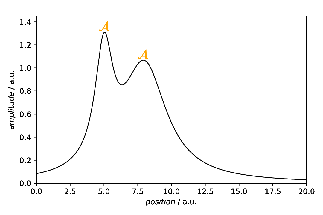
Fig. 33 Plot with markers using MathText (no LaTeX installation needed). Note that in this case, we set the edgewidth to zero, as otherwise, you get an effect similar to boldface. Furthermore, please note that in this particular case, you cannot have question marks surrounding the marker string, as otherwise, YAML is unhappy.
Markers using Unicode
Using the MathText feature of Matplotlib, even without LaTeX being installed, allows to even use Unicode symbols (using STIX fonts) as markers. One example inspired by the Matplotlib documentation, is given below.
239  - kind: singleplot
240    type: SinglePlotter1D
241    properties:
242      properties:
243        axes:
244          xlabel: "$position$ / a.u."
245          xlim: [0, 20]
246          ylim: [0, 1.45]
247      parameters:
248        tight_layout: True
249      filename: plotting-annotation-marker-unicode.pdf
250    apply_to:
251      - model_data
252    result:
253      - plot-with-marker-unicode
254    comment: >
255      Plotter that gets annotated later
256
257  - kind: plotannotation
258    type: Marker
259    properties:
260      parameters:
261        positions: peaks_xy
262        yoffset: 0.06
263        marker: "$\u266B$"
264      properties:
265        size: 14
266        edgewidth: 0
267        facecolor: blue
268    plotter: plot-with-marker-unicode
269    comment: >
270      Markers with default styling using Unicode (there is music in the peaks).
271
272      Note that in this case, you need to have question marks surrounding the
273      marker string, as otherwise, YAML is unhappy.
The resulting figure is shown below:
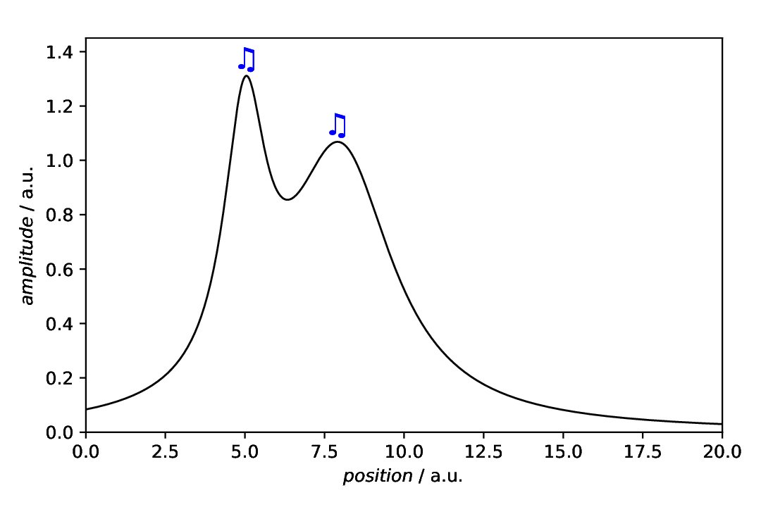
Fig. 34 Plot with markers using MathText (no LaTeX installation needed) to produce Unicode. Note that in this case, we set the edgewidth to zero, as otherwise, you get an effect similar to boldface. Furthermore, please note that in this particular case, you need to have question marks surrounding the marker string, as otherwise, YAML is unhappy.
This concludes our tour de force through using different kinds of markers.
Comments
As usual, a model dataset is created at the beginning, to have something to show. Here, a CompositeModel comprising of two Lorentizans is used to get two peaks that can be labelled.
For simplicity, a generic plotter is used, to focus on the annotations.
The sequence of defining plot and annotation(s) does not matter. You only need to provide the
resultkey with a unique name for whichever task you define first, to refer to it in the later task(s).Styling the marker, as shown here once for pure demonstration purposes, shall be used carefully in scientific presentations, but can nevertheless be very helpful.