You're reading the documentation for a development version. For the latest released version, please have a look at v0.10.
Plot annotations: Text (with lines)
Classes used:
Models:
Analysis:
Plotting:
Annotations:
Graphical representation of data and results is one of the most important aspects of presenting scientific results. A good figure is a figure allowing the reader to immediately catch the important aspects, not relying on reading the (nevertheless always important) caption with more description.
To this end, there is the frequent need to annotate figures, i.e. add additional lines, areas, or even text. This is what can be done with the concrete subclasses of aspecd.annotation.PlotAnnotation.
Here, we focus on simple text and text with attached lines added to a plot that are often used to label peaks. Note that these two kinds of annotations are quite different, although both involve text labels at given positions.
Recipe
Shown below is the entire recipe. As this is quite lengthy, separate parts will be detailed below in the “Results” section.
  1format:
  2  type: ASpecD recipe
  3  version: '0.2'
  4
  5settings:
  6  autosave_plots: False
  7
  8tasks:
  9  - kind: model
 10    type: Zeros
 11    properties:
 12      parameters:
 13        shape: 1001
 14        range: [0, 20]
 15    result: dummy
 16
 17  - kind: model
 18    type: CompositeModel
 19    from_dataset: dummy
 20    properties:
 21      models:
 22        - Lorentzian
 23        - Lorentzian
 24      parameters:
 25        - position: 5
 26          width: 0.8
 27        - position: 8
 28          width: 2
 29    result: model_data
 30
 31  - kind: singleanalysis
 32    type: PeakFinding
 33    apply_to: model_data
 34    result: peaks
 35
 36  - kind: singleplot
 37    type: SinglePlotter1D
 38    properties:
 39      properties:
 40        axes:
 41          xlabel: "$position$ / a.u."
 42          xlim: [0, 20]
 43          ylim: [0, 1.35]
 44        grid:
 45          show: True
 46          axis: x
 47          lines:
 48            linestyle: ":"
 49      parameters:
 50        tight_layout: True
 51      filename: plotting-annotation-text.pdf
 52    apply_to:
 53      - model_data
 54    result:
 55      - plot-with-text
 56    comment: >
 57      Plotter that gets annotated later
 58
 59  - kind: plotannotation
 60    type: Text
 61    properties:
 62      parameters:
 63        xpositions: peaks
 64        ypositions: 0.02
 65        texts:
 66          - "Peak a"
 67          - "Peak b"
 68      properties:
 69        color: red
 70        fontsize: smaller
 71        fontstyle: italic
 72        horizontalalignment: center
 73    plotter: plot-with-text
 74    comment: >
 75      Text labels at the bottom of the line to highlight the peaks.
 76
 77  - kind: plotannotation
 78    type: TextWithLine
 79    properties:
 80      parameters:
 81        xpositions: peaks
 82        ypositions:
 83          - 1.35
 84          - 1.12
 85        offsets:
 86          - [-0.5, 0.2]
 87          - [0.5, 0.2]
 88        texts:
 89          - "Peak a"
 90          - "Peak b"
 91      properties:
 92        text:
 93          color: green
 94          fontsize: larger
 95          fontstyle: italic
 96        line:
 97          edgecolor: blue
 98          linewidth: 0.8
 99    result: text-with-line
100    comment: >
101      Texts with attached lines. Due to the offset, you get "hooks"
102
103  - kind: singleplot
104    type: SinglePlotter1D
105    properties:
106      properties:
107        axes:
108          xlabel: "$position$ / a.u."
109          xlim: [0, 20]
110          ylim: [0, 1.7]
111      parameters:
112        tight_layout: True
113      filename: plotting-annotation-text-with-line.pdf
114    apply_to:
115      - model_data
116    annotations:
117      - text-with-line
118    comment: >
119      Plotter with annotations
120
121  - kind: singleanalysis
122    type: PeakFinding
123    properties:
124      parameters:
125        return_intensities: True
126    apply_to: model_data
127    result: peaks_with_intensities
128
129  - kind: plotannotation
130    type: TextWithLine
131    properties:
132      parameters:
133        positions: peaks_with_intensities
134        offsets:
135          - [-0.5, 0.2]
136          - [0.5, 0.2]
137        texts:
138          - "Peak a"
139          - "Peak b"
140      properties:
141        text:
142          color: green
143          fontsize: larger
144          fontstyle: italic
145        line:
146          edgecolor: blue
147          linewidth: 0.8
148    result: text-with-line-automatically-positioned
149    comment: >
150      Texts with attached lines. Due to the offset, you get "hooks"
151
152  - kind: singleplot
153    type: SinglePlotter1D
154    properties:
155      properties:
156        axes:
157          xlabel: "$position$ / a.u."
158          xlim: [0, 20]
159          ylim: [0, 1.7]
160      parameters:
161        tight_layout: True
162      filename: plotting-annotation-text-with-line-autopositioned.pdf
163    apply_to:
164      - model_data
165    annotations:
166      - text-with-line-automatically-positioned
167    comment: >
168      Plotter with annotations
Results
Examples for the figures created in the recipe are given below. While in the recipe, the output format has been set to PDF, for rendering them here they have been converted to PNG.
As this is a rather lengthy recipe demonstrating different scenarios, the individual cases are shown separately, each with the corresponding section of the recipe.
Text
The scenario: We have a curve comprising of two overlapping Lorentzians and want to highlight the peaks. Using the aspecd.analysis.PeakFinding analysis step allows us to place the labels at the correct x positions.
Here, we first plot the data, and afterwards annotate the plot with an annotation. This is why the plot task as a result set with its result key that is referred to in the annotation task with the plotter key.
36  - kind: singleplot
37    type: SinglePlotter1D
38    properties:
39      properties:
40        axes:
41          xlabel: "$position$ / a.u."
42          xlim: [0, 20]
43          ylim: [0, 1.35]
44        grid:
45          show: True
46          axis: x
47          lines:
48            linestyle: ":"
49      parameters:
50        tight_layout: True
51      filename: plotting-annotation-text.pdf
52    apply_to:
53      - model_data
54    result:
55      - plot-with-text
56    comment: >
57      Plotter that gets annotated later
58
59  - kind: plotannotation
60    type: Text
61    properties:
62      parameters:
63        xpositions: peaks
64        ypositions: 0.02
65        texts:
66          - "Peak a"
67          - "Peak b"
68      properties:
69        color: red
70        fontsize: smaller
71        fontstyle: italic
72        horizontalalignment: center
73    plotter: plot-with-text
74    comment: >
75      Text labels at the bottom of the line to highlight the peaks.
As we got the x positions for our text labels from the analysis step (PeakFinding), we use the xpositions``and ``ypositions keys here, rather than the simple positions key. Furthermore, as we want to have both labels appear with the same y position, we can provide a scalar here for the key ypositions. Of course, texts needs to be a list as well, with the same length as the positions.
The appearance of the text can be controlled in quite some detail. For the styling available, see the documentation of the aspecd.plotting.TextProperties class - and use sparingly in scientific context. After all, it is science, not pop art. One particularly important setting here is the horizontal alignment using the horizontalalignment key: Typically, you want to have your text labels in such case be centred horizontally.
The resulting figure is shown below:
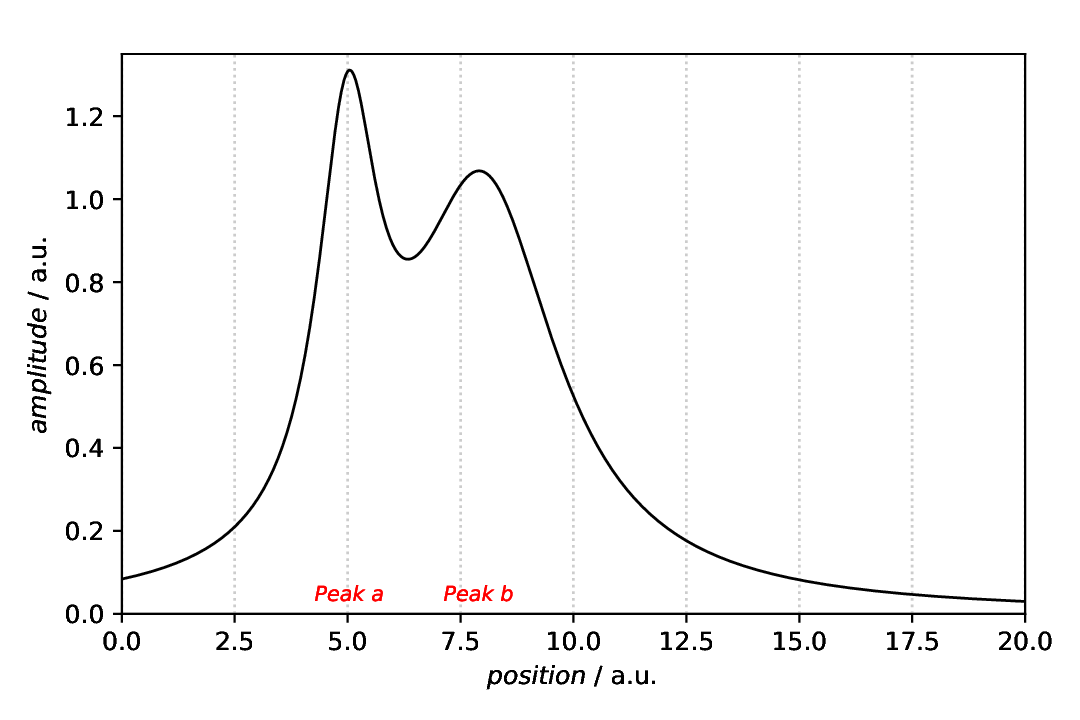
Fig. 25 Plot with two text labels for the peak positions as annotation. While not always sensible in scientific context, the text has been styled here, using a different colour, font size and font style. Note that in this case, the plot(ter) has been defined first, with a result key for later reference, and the annotation afterwards, referring to the plotter using the plotter key.
To demonstrate that the labels are indeed horizontally centred about the peaks, a grid (vertical dotted lines) has been added as guide for the eye of the reader in this case.
Text with lines
The scenario is the same as above: We have a curve comprising of two overlapping Lorentzians and want to highlight the peaks. Using the aspecd.analysis.PeakFinding analysis step allows us to place the labels at the correct x positions.
Here, we first create the annotation and afterwards plot the data and annotate the plot with this annotation. This is why the annotation task as a result set with its result key that is referred to in the plotter task with the annotations key. Mind the plural here, as a plot can be annotated with more than one annotation.
 76  - kind: plotannotation
 77    type: TextWithLine
 78    properties:
 79      parameters:
 80        xpositions: peaks
 81        ypositions:
 82          - 1.35
 83          - 1.12
 84        offsets:
 85          - [-0.5, 0.2]
 86          - [0.5, 0.2]
 87        texts:
 88          - "Peak a"
 89          - "Peak b"
 90      properties:
 91        text:
 92          color: green
 93          fontsize: larger
 94          fontstyle: italic
 95        line:
 96          edgecolor: blue
 97          linewidth: 0.8
 98    result: text-with-line
 99    comment: >
100      Texts with attached lines. Due to the offset, you get "hooks"
101
102  - kind: singleplot
103    type: SinglePlotter1D
104    properties:
105      properties:
106        axes:
107          xlabel: "$position$ / a.u."
108          xlim: [0, 20]
109          ylim: [0, 1.7]
110      parameters:
111        tight_layout: True
112      filename: plotting-annotation-text-with-line.pdf
113    apply_to:
114      - model_data
115    annotations:
116      - text-with-line
117    comment: >
118      Plotter with annotations
As we got the x positions for our text labels from the analysis step (PeakFinding), we use the xpositions``and ``ypositions keys here, rather than the simple positions key. In this case, we want to have the labels appear close to the actual line, hence with different y positions. Therefore, the ypositions key contains a list. Of course, texts needs to be a list as well, with the same length as the positions.
The appearance of the text and connecting lines can be controlled in quite some detail. For the styling available, see the documentation of the aspecd.plotting.AnnotationProperties class - and use sparingly in scientific context. After all, it is science, not pop art. Note that you cannot set the text alignment for this type of annotations, as it gets set automatically for you depending on the horizontal offset between the position and the text label.
The resulting figure is shown below:
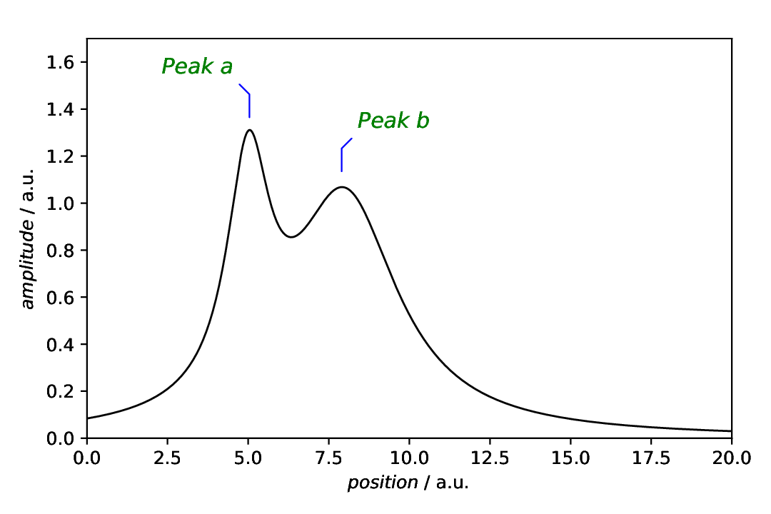
Fig. 26 Plot with two text labels with attached lines for the peak positions as annotation. Note that in this case, the annotation has been defined first, with a result key for later reference, and the plot(ter) afterwards, referring to the annotation using the annotations key. Mind the plural here, as a plotter can have multiple annotations.
Text with lines - automatically positioned
In the example above, we have shown how to automatically position the lines at the peak positions in the x direction, but still have positioned the annotations in the y direction manually. How about getting both, x and y position of the peaks automatically, and only providing the (relative) offset for the text labels?
This is possible by using a new feature of the aspecd.analysis.PeakFinding class, namely to explicitly return the intensities as well. Thus, you get a two-dimensional (two-column) numpy array with the peak positions (x values) in the first and the peak intensities (y values) in the second column. This can nicely be used to directly feed it into the positions key of the annotation;
121  - kind: singleanalysis
122    type: PeakFinding
123    properties:
124      parameters:
125        return_intensities: True
126    apply_to: model_data
127    result: peaks_with_intensities
128
129  - kind: plotannotation
130    type: TextWithLine
131    properties:
132      parameters:
133        positions: peaks_with_intensities
134        offsets:
135          - [-0.5, 0.2]
136          - [0.5, 0.2]
137        texts:
138          - "Peak a"
139          - "Peak b"
140      properties:
141        text:
142          color: green
143          fontsize: larger
144          fontstyle: italic
145        line:
146          edgecolor: blue
147          linewidth: 0.8
148    result: text-with-line-automatically-positioned
149    comment: >
150      Texts with attached lines. Due to the offset, you get "hooks"
151
152  - kind: singleplot
153    type: SinglePlotter1D
154    properties:
155      properties:
156        axes:
157          xlabel: "$position$ / a.u."
158          xlim: [0, 20]
159          ylim: [0, 1.7]
160      parameters:
161        tight_layout: True
162      filename: plotting-annotation-text-with-line-autopositioned.pdf
163    apply_to:
164      - model_data
165    annotations:
166      - text-with-line-automatically-positioned
167    comment: >
168      Plotter with annotations
The result is fairly similar to the result shown above with the manual positioning, but this time, we need not care of the y positions by ourselves. Use whatever suits your needs in the given situation.
The resulting figure is shown below:
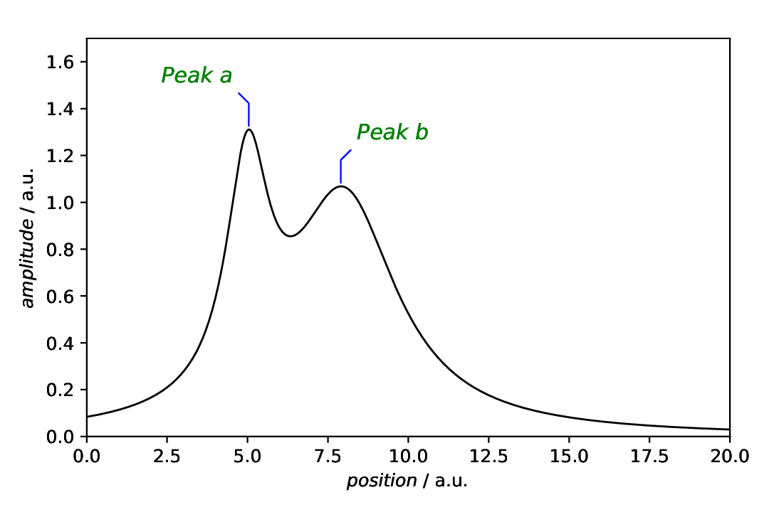
Fig. 27 Plot with two text labels with attached lines for the peak positions as annotation. Note that in this case, the annotation has been defined first, with a result key for later reference, and the plot(ter) afterwards, referring to the annotation using the annotations key. Mind the plural here, as a plotter can have multiple annotations. Furthermore, instead of only providing the xpositions by the result of the PeakFinding analysis step, we got both, x and y positions, and thus used the positions key instead.
Comments
As usual, a model dataset is created at the beginning, to have something to show. Here, a CompositeModel comprising of two Lorentizans is used to get two peaks that can be labelled.
For simplicity, a generic plotter is used, to focus on the annotations.
The sequence of defining plot and annotation(s) does not matter. You only need to provide the
resultkey with a unique name for whichever task you define first, to refer to it in the later task(s).Styling the text (and lines), as shown here for pure demonstration purposes, shall be used carefully in scientific presentations, but can nevertheless be very helpful.